Dense Text Is Harder to Reconstruct
This is a follow-up to Part 1: Do Transformers Feel the Density of Text?
In Part 1, we observed the forward pass of transformers. In an Encoder (BERT), the Layer Delta of high-density sentences was larger. In a Decoder (Qwen3), it was surprisingly smaller. Surprisal analysis explained the reversal: dense sentences distribute information uniformly across tokens (the UID hypothesis), which keeps per-token state changes steady rather than spiking.
But all of that was observation. We watched models read.
This time we change the game entirely. We destroy a sentence completely, then try to rebuild it from scratch.
What Is a Diffusion Language Model?
If you have used image-generation AI like Stable Diffusion or DALL-E, you already know the core idea: start from noise, and gradually denoise until a coherent output emerges. The same principle applies to text.
Discrete Diffusion (D3PM; Austin et al., 2021) defines a diffusion process over discrete token spaces. In the absorbing-state variant, the forward process independently transitions each token toward a single absorbing state, $[\text{MASK}]$:
$$q(x_t \mid x_0) = \text{Cat}\bigl(x_t;; (1-\beta_t),\mathbf{e}{x_0} + \beta_t,\mathbf{e}{[\text{MASK}]}\bigr)$$
Here $\beta_t$ is the noise schedule and $\mathbf{e}$ denotes a one-hot vector. As $t \to T$, every token converges to $[\text{MASK}]$ --- the sentence is obliterated into a blank canvas.
The reverse process uses a model $p_\theta(x_0 \mid x_t)$ at each step to predict the original token at each masked position:
$$p_\theta(x_{t-1} \mid x_t) = \sum_{x_0} q(x_{t-1} \mid x_t, x_0), p_\theta(x_0 \mid x_t)$$
If we record the model’s confidence and uncertainty at every step, we can watch the sentence crystallize from noise into text.
The crystallization hypothesis: Dense sentences are harder to reconstruct. They remain uncertain for more steps.
BERT as a Discrete Diffusion Denoiser
Ideally, we would use a purpose-built diffusion language model. MDLM (Sahoo et al., 2024) is the leading option --- 169.6 million parameters, trained with a continuous-time noise schedule on OpenWebText. But its codebase is hard-wired to flash_attn and triton, both NVIDIA CUDA-only libraries. The DiT backbone calls torch.cuda.amp; the DiMamba backbone requires mamba_ssm + triton. BD3-LM shares the same codebase. None of them run on Apple Silicon (MPS).
So we used an alternative: BERT as a discrete diffusion denoiser.
This is not a hack. In an absorbing-state D3PM, the core computation of the reverse step is $p_\theta(x_0 \mid x_t)$ --- predicting the original token at each masked position. This is exactly BERT’s Masked Language Modeling (MLM) objective:
$$\mathcal{L}{\text{MLM}} = -\mathbb{E}{i \in \mathcal{M}} \bigl[\log P_\theta(x_i \mid \mathbf{x}_{\backslash \mathcal{M}})\bigr]$$
where $\mathcal{M}$ is the set of masked positions. BERT’s $[\text{MASK}]$ prediction is a denoising step.
MDLM itself uses this structure --- it adds a learned continuous-time noise schedule $\beta(t)$, but the core mechanism is the same masked-token prediction. The theoretical equivalence between MLM and absorbing-state D3PM is well established.
We used klue/bert-base for Korean and bert-base-uncased for English as iterative unmasking engines.
Extracting Crystallization Trajectories
For a sentence $s = (t_1, \ldots, t_S)$:
- Mask everything. Replace all content tokens with $[\text{MASK}]$: $x^{(0)} = ([\text{MASK}], \ldots, [\text{MASK}])$.
- Predict. At each step $k$, the model predicts a probability distribution $P_\theta(v \mid x^{(k)})$ for every position $i$.
- Record. We log the confidence and entropy at each position:
$$c_i^{(k)} = \max_v P_\theta(v \mid x^{(k)}) \qquad H_i^{(k)} = -\sum_v P_\theta(v \mid x^{(k)}) \log_2 P_\theta(v \mid x^{(k)})$$
- Unmask the most confident. Among still-masked positions, the one with the highest $c_i^{(k)}$ gets unmasked: $x_i^{(k+1)} = \arg\max_v P_\theta(v \mid x^{(k)})$.
- Repeat until every token is restored ($k = 1, \ldots, K$ where $K = S$).
This produces a denoising heatmap for each sentence. The x-axis is token position $i$, the y-axis is denoising step $k$. Color represents entropy $H_i^{(k)}$ --- bright means high uncertainty, dark means resolved.
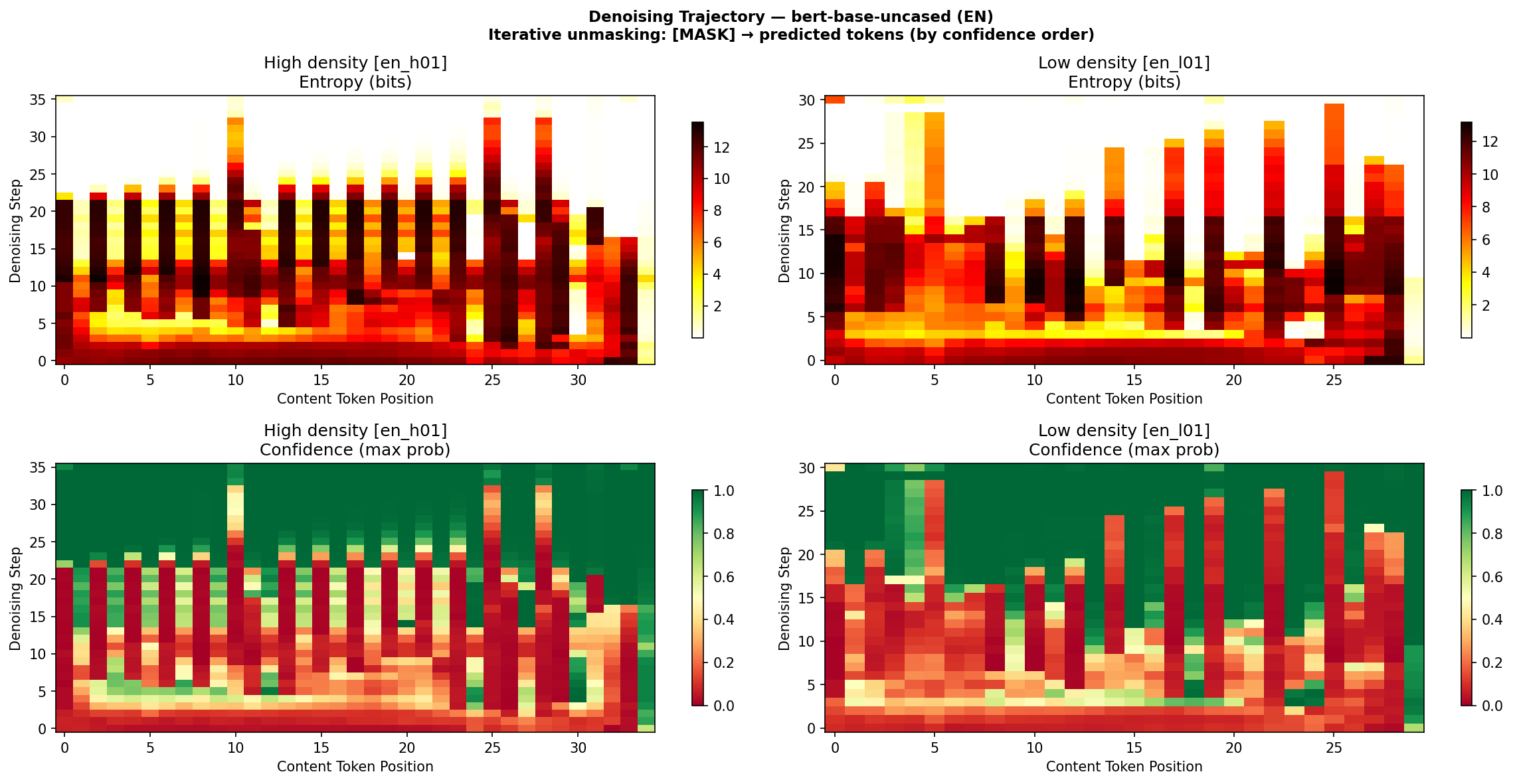 Figure 1: Denoising heatmap from bert-base-uncased on English sentences. Top: entropy, bottom: confidence. The high-density sentence (left) maintains uncertainty longer.
Two Metrics: Crystallization and Convergence
We measured two quantities from these trajectories.
Mean Crystallization ($\bar{\kappa}$) --- the crystallization point $\kappa_i$ of token $i$ is the step number at which it gets unmasked. The sentence-level metric normalizes by total steps:
$$\bar{\kappa} = \frac{1}{S}\sum_{i=1}^{S} \frac{\kappa_i}{K}$$
$\bar{\kappa} \approx 0$ means most tokens were resolved immediately. $\bar{\kappa} \approx 1$ means the model stayed uncertain until the very end.
Convergence Area ($A$) --- the area under the mean entropy curve over the entire denoising trajectory. This captures the total uncertainty the model experienced during reconstruction:
$$A = \int_0^1 \bar{H}(t), dt, \qquad \bar{H}(t) = \frac{1}{S}\sum_{i=1}^{S} H_i^{(\lfloor tK \rfloor)}$$
A large $A$ means the model’s uncertainty remained high for a long time --- the sentence was hard to reconstruct.
Pilot Results (n = 5 per Group)
We began with 5 high-density and 5 low-density sentences per language, the same set from Part 1.
| Model | Metric | Direction | p-value |
|---|---|---|---|
| klue/bert-base (KO) | Mean crystallization | No difference | 1.00 ns |
| klue/bert-base (KO) | Convergence area | No difference | 0.67 ns |
| bert-base-uncased (EN) | Mean crystallization | No difference | 0.67 ns |
| bert-base-uncased (EN) | Convergence area | High > Low | 0.011* |
One signal survived. English high-density sentences had significantly larger convergence area. When the model tried to reconstruct a dense English sentence, it experienced more total uncertainty across the entire denoising trajectory. More information packed into the sentence means more positions where the model hesitates --- “what goes here?” is a harder question when the answer carries more meaning.
Korean showed nothing. We will come back to that.
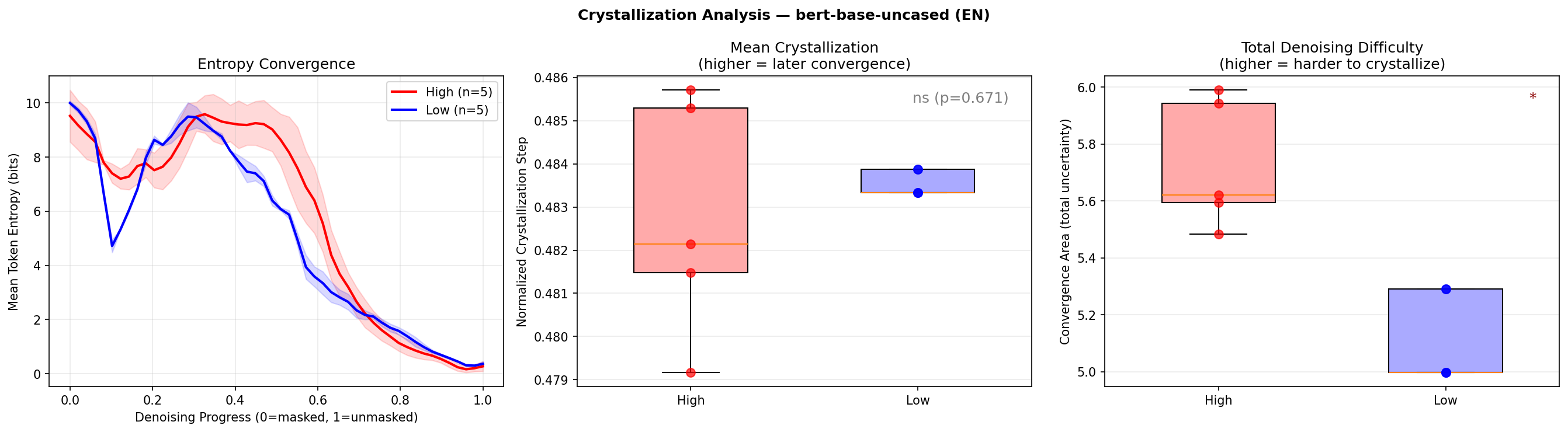 Figure 2: Entropy convergence curves and crystallization distribution for English sentences. High-density sentences (red) show larger convergence area.
From Pilot to Validation
Five sentences per group is a whisper of evidence. We needed to shout.
Two problems haunted the pilot:
- Sample size. $n = 5$ means any single outlier sentence dominates the result. Even a significant p-value comes with a wide confidence interval.
- Confounding. High-density sentences were literary aphorisms; low-density sentences were everyday descriptions. A probing classifier achieved 100% accuracy at every layer, but PCA showed this was trivially driven by vocabulary and style --- not density itself.
We addressed both problems simultaneously.
Validation Experiment 1: Expanded Corpus (100 Sentences)
We scaled to 25 high-density and 25 low-density sentences per language (100 total). This increased statistical power by 5x.
Validation Experiment 2: Minimal Pairs (100 Pairs)
To isolate density from vocabulary and style confounds, we constructed 100 minimal pairs --- 50 per language. Each pair expresses the same meaning at two density levels: a compressed (high-density) version and an expanded (low-density) version.
Korean examples:
| Low density (expanded) | High density (compressed) |
|---|---|
| If you don’t prepare enough before a presentation, it’s hard to answer properly when you get questions | An unprepared presentation crumbles at the first question |
| If you update the system without backing up your files, you may lose important documents | An update without backup invites data loss |
| If you leave a small crack in the window alone, it’ll gradually grow until the glass breaks | A neglected crack eventually shatters the pane |
Same proposition, different compression. If the model’s internal signals still differ between high and low density here, it cannot be due to vocabulary or topic --- it must be responding to the compression itself.
We used Mann-Whitney $U$ tests for the expanded corpus and Wilcoxon signed-rank tests for minimal pairs.
Validation Results
This is the critical update from the pilot. All three paradigm signals were tested: Layer Delta (Encoder), Surprisal CV (Decoder), and Convergence Area (Diffusion).
Expanded Corpus (general.csv)
| Signal | Language | Direction | p-value |
|---|---|---|---|
| Layer Delta | KO | High > Low | .003** |
| Layer Delta | EN | High > Low | .0001*** |
| Surprisal Mean | KO | High > Low | <.0001*** |
| Surprisal Mean | EN | High > Low | <.0001*** |
| Surprisal CV | KO | High < Low | <.0001*** |
| Surprisal CV | EN | High < Low | .003** |
| Convergence Area | KO | --- | .94 ns |
| Convergence Area | EN | High > Low | <.0001*** |
Every signal that was marginally significant or nonsignificant in the pilot lit up with the larger sample. English Layer Delta went from nonsignificant to $p = .0001$. English Surprisal CV went from nonsignificant to $p = .003$. English Convergence Area went from $p = .011$ to $p < .0001$.
Korean Convergence Area remained stubbornly null ($p = .94$). More on that shortly.
Minimal Pairs
| Signal | Language | Direction | p-value |
|---|---|---|---|
| Layer Delta | KO | High > Low | .005** |
| Layer Delta | EN | High > Low | <.0001*** |
| Surprisal Mean | KO | High > Low | <.0001*** |
| Surprisal Mean | EN | High > Low | <.0001*** |
| Surprisal CV | KO | High < Low | <.0001*** |
| Surprisal CV | EN | High < Low | <.0001*** |
| Convergence Area | KO | --- | .44 ns |
| Convergence Area | EN | High > Low | <.0001*** |
Even when meaning is held constant and only compression varies, the same pattern holds. This is not a vocabulary artifact. The model is responding to density itself.
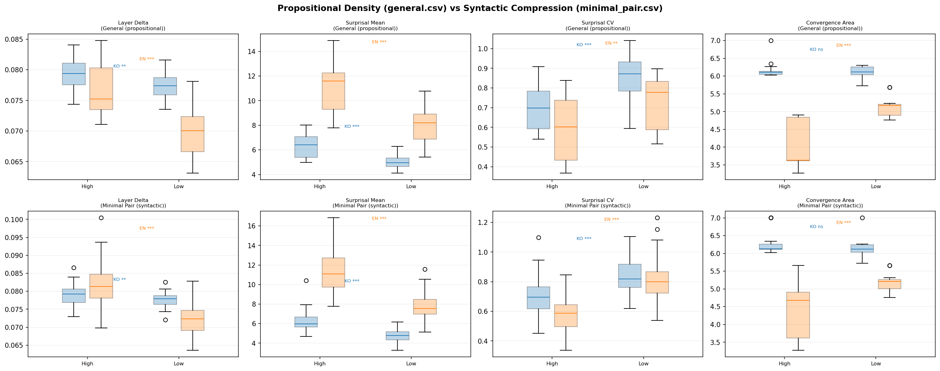 Figure 3: Propositional density (general) vs syntactic compression (minimal pair) — English convergence area is significant in both conditions.
Cross-Signal Correlation: Prediction Difficulty Equals Reconstruction Difficulty
One of the most striking findings emerged from the correlation analysis between signals across paradigms.
In English, we found a strong negative correlation between surprisal mean (Decoder signal) and convergence area (Diffusion signal):
$$\rho = -0.624, \quad p < .0001 \text{ (***)}$$
What does this mean? Sentences that are harder for a Decoder to predict (high surprisal) are also harder for a Diffusion model to reconstruct (high convergence area). The negative sign arises because the Decoder measures “surprise per token” while the Diffusion process measures “total residual entropy” --- both capture difficulty, but from opposite ends of the generation process.
Prediction difficulty approximates reconstruction difficulty. A sentence that makes a left-to-right model say “I didn’t see that coming” at every token is the same sentence that makes a denoising model say “I still can’t figure out what goes here” for many steps.
In Korean, a different cross-signal emerged: Layer Delta and surprisal mean showed a significant positive correlation ($\rho = 0.378$, $p = .007$). Sentences that require more representational transformation across layers (higher Layer Delta) are the same sentences that carry more information per token (higher mean surprisal).
These cross-paradigm correlations confirm that the three signals are not independent flukes. They form a coherent system: different instruments measuring the same underlying property.
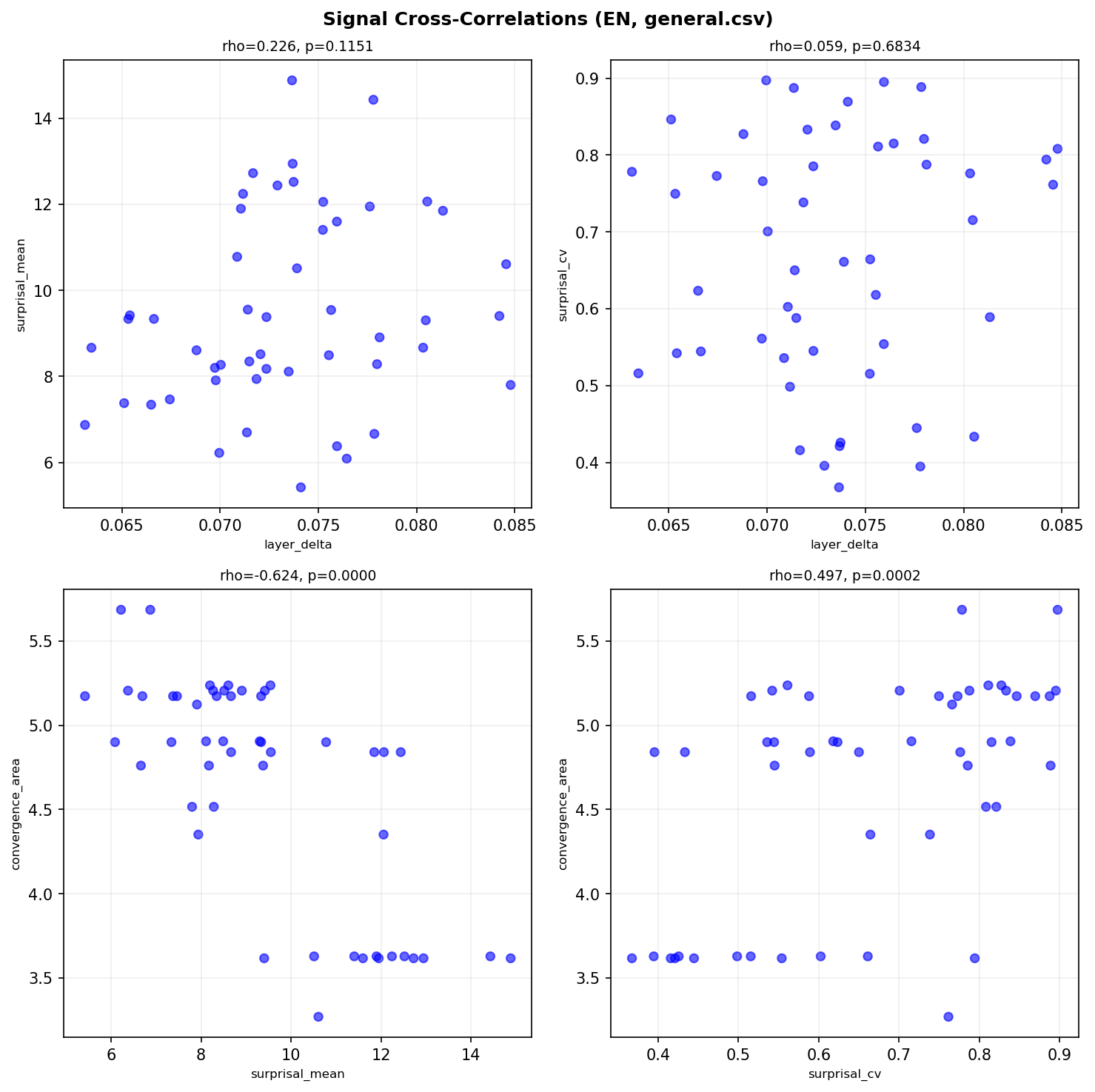 Figure 4: English signal cross-correlations. Surprisal Mean ↔ Convergence Area (ρ=-0.624**) confirms ‘prediction difficulty ≈ reconstruction difficulty.’*
Why Korean Diffusion Results Are Null
Korean Convergence Area was nonsignificant in every experiment: $p = .67$ (pilot), $p = .94$ (expanded corpus), $p = .44$ (minimal pairs). This is not a power issue --- the expanded corpus had 50 sentences per group, and the other signals (Layer Delta, Surprisal) were highly significant for Korean.
Three hypotheses:
1. SOV structure disrupts unmasking order. Korean is a verb-final (SOV) language. In iterative unmasking, the model restores the most confident position first. In Korean, content words (nouns, adjectives) tend to be restored early, while particles and verb endings come last. This unmasking order may be driven by morphosyntactic predictability rather than semantic density. The trajectory looks the same regardless of whether the sentence is dense or sparse, because the reconstruction bottleneck is always at the grammatical endings, not the content-bearing positions.
2. BERT’s MLM head insensitivity. The klue/bert-base model shows density sensitivity in its internal representations (Layer Delta is significant), but its output layer --- the MLM head that predicts token probabilities --- may not reflect this sensitivity. The internal representations “feel” density, but the decoder head projects this into a space where the density signal washes out.
3. Korean morphological complexity. Korean agglutinative morphology means a single “token” can encode multiple grammatical relations. The entropy at each masked position is dominated by the combinatorial explosion of possible suffixes, overwhelming the subtler signal of semantic density.
The Korean null result is not a failure --- it is an asymmetry that demands explanation. And the fact that the same Korean sentences produce highly significant results for Layer Delta ($p = .005$) and Surprisal CV ($p < .0001$) means density is not invisible to the model. It simply does not manifest in the diffusion trajectory.
The Complete Picture: Three Paradigms, One Property
We can now assemble the full validated results across all three transformer paradigms:
| Paradigm | Signal | KO gen. | KO pair | EN gen. | EN pair |
|---|---|---|---|---|---|
| Encoder | Layer $\delta$ | .003** | .005** | .0001*** | <.0001*** |
| Decoder | Surprisal CV | <.0001*** | <.0001*** | .003** | <.0001*** |
| Diffusion | Convergence $A$ | .94 ns | .44 ns | <.0001*** | <.0001*** |
Each paradigm detects density through its own internal signature:
Encoder (BERT, bidirectional): The model sees the entire sentence at once. High-density sentences require more representational transformation between layers --- the Layer Delta is larger. Intuitively, unpacking compressed meaning demands more work at each processing step. Every layer must do heavier lifting to decompose the tightly packed semantics.
Decoder (Qwen3, causal): The model processes tokens left to right. High-density sentences have more uniform surprisal --- the coefficient of variation is lower. This aligns with the Uniform Information Density (UID) hypothesis (Levy & Jaeger, 2007): well-written dense text distributes information evenly across tokens. There are no “throwaway” tokens and no sudden spikes. Every token carries its share.
Diffusion (BERT as denoiser): The model destroys the sentence entirely and rebuilds it from nothing. For English, high-density sentences generate more total uncertainty during reconstruction --- the convergence area is larger. The sentence lingers in an ambiguous state longer because each position has more possible completions that are consistent with the emerging context.
Three different angles. Three different computational metaphors. And they all converge on the same conclusion: density is harder.
But “harder” means different things depending on the paradigm:
- For the Encoder: “more transformation is needed”
- For the Decoder: “prediction is uniformly difficult”
- For the Diffusion model: “reconstruction stays uncertain longer”
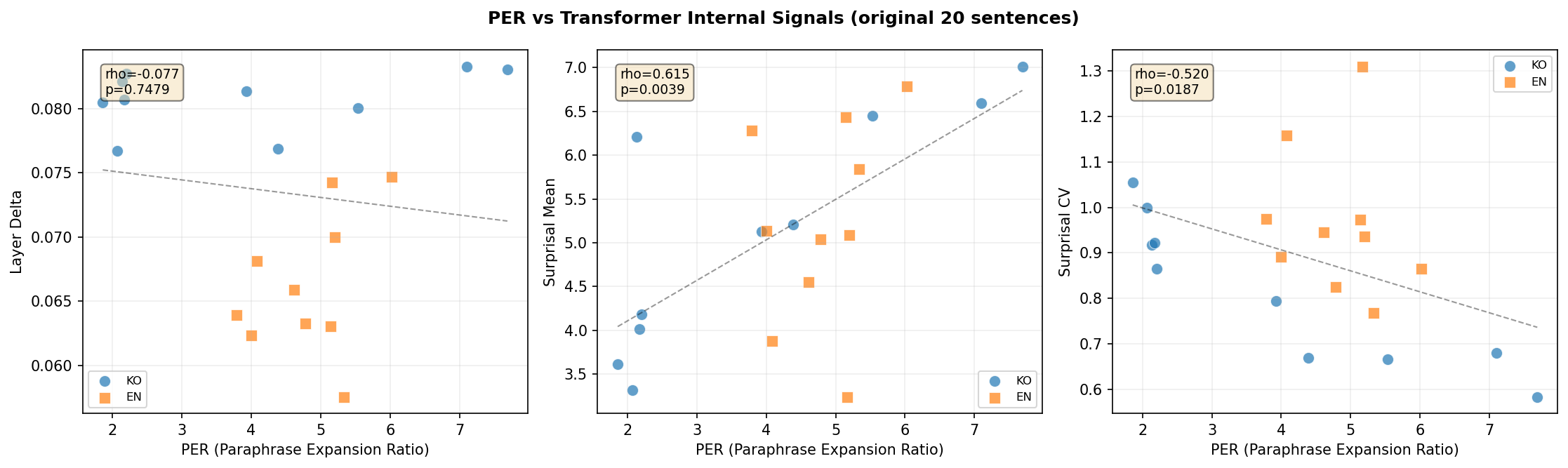 Figure 5: PER vs internal signals. Higher PER correlates with higher surprisal (ρ=0.867) and lower CV (ρ=-0.952).
What This Study Does Not Answer
Korean diffusion asymmetry. We have hypotheses for why Korean convergence area is null, but no definitive explanation. A controlled experiment with MDLM on CUDA hardware, or a systematic comparison of SVO vs SOV languages, would help.
True diffusion language models. BERT iterative unmasking is theoretically equivalent to absorbing-state D3PM, but it is not identical to a model trained with a continuous noise schedule. The comparison with MDLM (or newer models) awaits CUDA GPU access.
Causality. We observed that density correlates with these internal signals. We did not prove that density causes them. A sentence can be dense and also stylistically marked, topically specialized, or syntactically complex. The minimal pair experiment controls for meaning, but not for all possible confounds. A factorial design crossing density with difficulty, register, and genre would be needed to isolate causal contributions.
PER standardization. Our density metric (Paraphrase Expansion Ratio) depends on which LLM performs the paraphrase. In Part 1, we showed that GPT/Claude models agree on density rankings ($\rho = 0.74$—$0.88$) while Gemini diverges. PER is a useful ordinal measure, but it is not yet a calibrated instrument.
Closing Thoughts
People struggle with dense text too. When you read Burckhardt’s “If a revolution does not make its sworn enemy its master, that alone is good fortune,” you pause. You reread. You reach for your own experience to make sense of the claim. The sentence is short, but the unpacking is long.
Transformers do something structurally analogous. The Encoder’s large Layer Delta is the computational equivalent of “thinking harder at each layer.” The Decoder’s uniform surprisal is the trace of a sentence that distributes its cognitive load evenly, with no easy tokens to coast through. The Diffusion model’s high convergence area is the shadow of a sentence that resists being pinned down --- every masked position could plausibly be many things, and the model lingers in this ambiguity longer.
None of this is “understanding.” Models do not comprehend Burckhardt’s pessimism about revolution, or the irony of Shaw’s observation that people fear freedom. But density --- the property of packing more meaning into fewer tokens --- leaves a measurable trace in how these models process text. And the shape of that trace changes depending on the computational paradigm: simultaneous attention, sequential prediction, or noise-to-signal reconstruction.
The deepest finding might be the cross-signal correlation. The fact that prediction difficulty (Decoder) and reconstruction difficulty (Diffusion) are strongly correlated ($\rho = -0.624$, $p < .0001$) suggests that density is not an artifact of any single model architecture. It is a property of the text itself, visible from multiple computational vantage points.
Dense writing is compressed thought. And decompressing it --- whether you are a human rereading Burckhardt, a BERT model transforming representations layer by layer, a GPT-class model predicting one token at a time, or a diffusion process rebuilding a sentence from nothing --- takes proportionally more effort.
The effort is different in each case. But the proportionality is the same.